Start Python for Image Processing with OpenCV and ML -Part 4 Noise Removal
- 2023年5月25日
- 読了時間: 2分
更新日:2025年6月9日

Noise removal is an important practice of Computer Vision. As we have already known, the images we get in practice are not always clean as we expected. We could extract only the part we are interested in by using ROI, which was introduced in the last part. While, noise removal can be applied before getting ROIs or after getting ROIs in most cases to get a better result.
In OpenCV, we usually remove noises by blurring the picture and applying morphological operators.
Let us see an example.
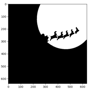
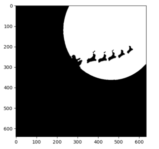
First, we have a picture as the left picture above and the mask by applying threshold as the right picture above. We could see starlight in the background.
When we blurred the picture by several methods, we could see the differences as below.

The first two methods actually get the same results. They applied an average blurring method to the image through a kernel.
Obviously, “medianBlur” and “GaussianBlur” get different results from the first two. Compared with average blurring, median blurring is stronger in visual presentation.
Gaussian blurring kept the edge clear to some degree, blurring applied though.
In this example, these 4 methods all did a good job in removing the starlight, while “bilateralFilter” kept the edges clear because it does not do average in the edge area. Therefore, it is used widely in edge detection.
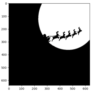
Furthermore, we might want to remove the shadow in the moon as well by using morphological operators. I will preprocess the image by median blur function above because it had a better result in this example.

Then we could remove noises by dilation, erosion, opening or closing.
Dilation is that white pixel points are dilated, while erosion is that white pixel points are eroded by black points, as the picture shows above. If we dilate the thresh picture again and again, we could certainly get a clear moon-liked shape area, but remember that we also modified the original contour position by doing so. And the same applies to erosion. The original contour will become smaller and smaller.
Therefore, what we could do is opening and closing, which are dilation after erosion and erosion after dilation respectively.
It is obvious that closing gives the similar result we expected, so we could adjust the parameter of kernel size and iterations, enhancing the effects.

We almost get what we want. In fact, there are also other flexible methods that we could customize to get a better result. If you have interests, please be sure to follow us for further information!
Please feel free to contact us if you have any comments.
Stay tuned for the next part, coming next month!


